Using pyirf to calculate IRFs from the FACT Open Data

Note In FACT, we used a different terminology, partly because of being a monoscopic telescope or out of confusion witht the CTA terms, in this context DL3 are reconstructed events, but not necessarily already with the IRF

import numpy as np
import astropy.units as u
import matplotlib.pyplot as plt
import subprocess as sp

%matplotlib inline

Download Data

path = "gamma_test_dl3.hdf5"
url = f"https://factdata.app.tu-dortmund.de/dl3/FACT-Tools/v1.1.2/{path}"
ret = sp.run(["curl", "-z", path, "-fsSLO", url], stdout=sp.PIPE, stderr=sp.PIPE, encoding='utf-8')
if ret.returncode != 0:
    raise IOError(ret.stderr)

Read in the data

from astropy.table import QTable
import astropy.units as u
import tables

Simulated Event Info

Currently, pyirf only works with powerlaw simulated events, like CORSIKA does it. We want to also support arbitrary histograms / event distributions, but that is not yet implemented.

This can be created from a file with that information, but I will just create it here.

from pyirf.simulations import SimulatedEventsInfo

simulation_info = SimulatedEventsInfo(
    energy_min=200 * u.GeV,
    energy_max=50 * u.TeV,
    spectral_index=-2.7,
    n_showers=12600000,
    max_impact=300 * u.m,
    viewcone_min=0 * u.deg,
    viewcone_max=0 * u.deg,
)

DL2 Event List

pyirf does not prescribe or use a specific DL2 file format. You need to read the data into an astropy.table.QTable following our conventions, detailed in the docs here:

https://cta-observatory.github.io/pyirf/introduction.html#dl2-event-lists

The FACT-Tools / aict-tools analysis chain uses a column-oriented hdf5 file written using h5py.

Unfortunately, units have to be known and are not in the metadata.

gammas = QTable()

# mapping of <target column name>: (<column in the file, unit>)
columns = {
    'obs_id': ('run_id', None),
    'event_id': ('event_num', None),
    'reco_energy': ('gamma_energy_prediction', u.GeV),
    'true_energy': ('corsika_event_header_total_energy', u.GeV),
    'true_az': ('source_position_az', u.deg),
    'pointing_az': ('pointing_position_az', u.deg),
    'theta': ('theta_deg', u.deg),
    'gh_score': ('gamma_prediction', None),
}

with tables.open_file('gamma_test_dl3.hdf5', mode='r') as f:
    events = f.root.events

    for col, (name, unit) in columns.items():
        if unit is not None:
            gammas[col] = u.Quantity(events[name][:], unit, copy=False)
        else:
            gammas[col] = events[name][:]

    gammas['true_alt'] = u.Quantity(90 - events['source_position_zd'][:], u.deg, copy=False)
    gammas['pointing_alt'] = u.Quantity(90 - events['pointing_position_zd'][:], u.deg, copy=False)


# make it display nice
for col in gammas.colnames:
    if gammas[col].dtype == float:
        gammas[col].info.format = '.2f'

gammas[:10]

QTable length=10

obs_id	event_id	reco_energy	true_energy	true_az	pointing_az	theta	gh_score	true_alt	pointing_alt
		GeV	GeV	deg	deg	deg		deg	deg
int64	int64	float64	float64	float64	float64	float64	float64	float64	float64
11583	403	638.00	712.87	353.00	349.76	1.49	0.45	79.34	79.33
106806	237	815.28	885.04	353.00	42.35	0.02	0.82	89.37	89.23
11325	166	838.62	928.05	353.00	-4.95	0.26	0.75	83.37	83.92
13486	165	680.72	420.22	353.00	348.77	0.13	0.78	81.92	82.02
14228	122	1896.68	2458.86	353.00	351.27	0.08	0.88	70.51	70.69
108312	221	4430.69	5347.98	353.00	-5.94	0.05	0.97	66.55	66.12
13327	310	3649.23	4550.83	353.00	347.98	0.04	0.91	83.53	83.75
107296	237	1723.47	2109.52	353.00	350.67	0.05	0.20	82.56	82.05
14269	217	956.90	953.94	353.00	-5.98	0.17	0.79	69.53	70.02
108669	183	804.27	626.66	353.00	-6.38	0.12	0.84	61.06	60.54

Apply Event Selection

We remove likely hadronic events by requiring a minimal gh_score.

We will calculate point-like IRFs, that means selecting events in a radius around the assumed source position.

gammas['selected_gh'] = gammas['gh_score'] > 0.8
gammas['selected_theta'] = gammas['theta'] < 0.16 * u.deg

gammas['selected'] = gammas['selected_gh'] & gammas['selected_theta']

np.count_nonzero(gammas['selected']) / len(gammas)

0.18115575805640652

Calculate IRFs

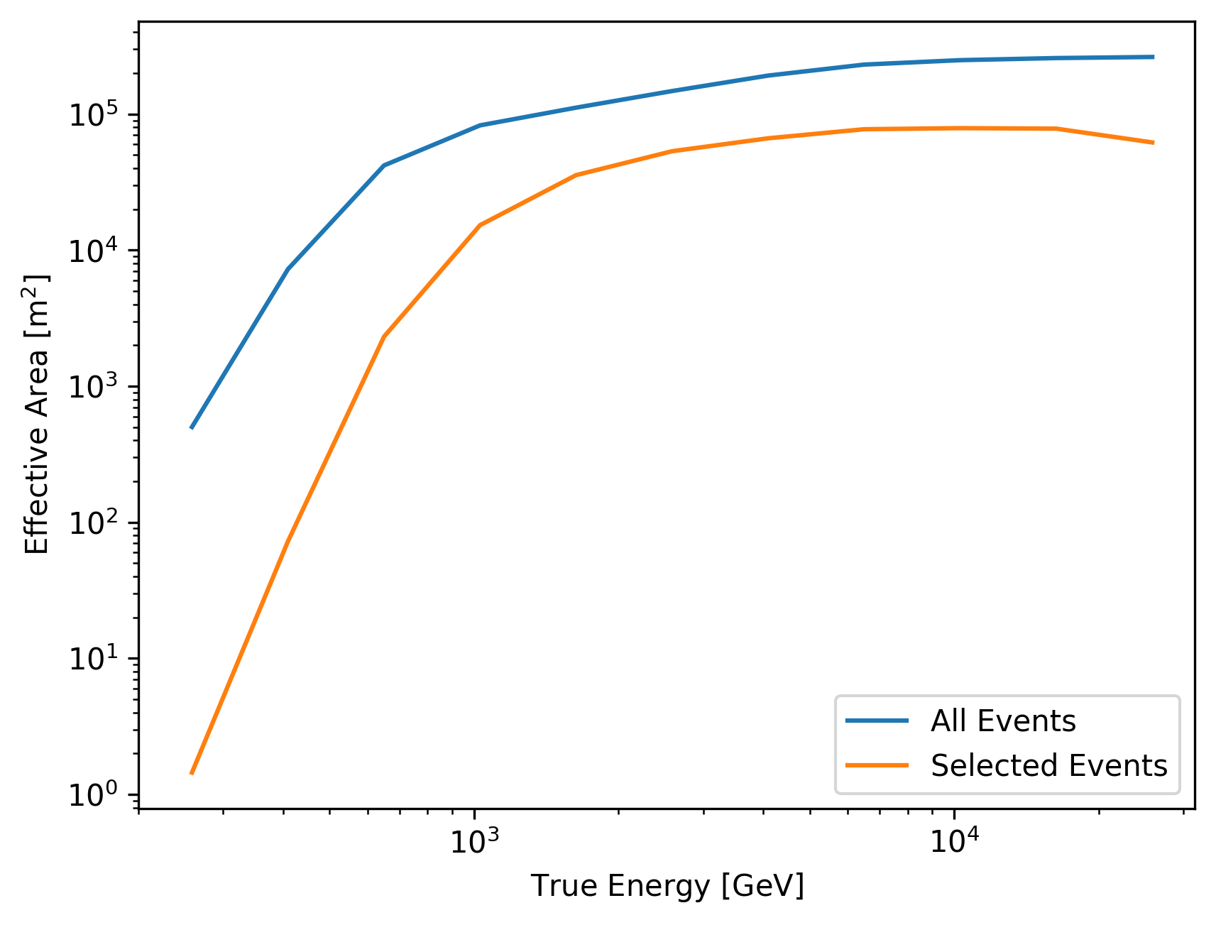
Effective area

We only have point-like simulations at a specific wobble offset (0.6° for FACT), so we calculate the effective area for all events at once, equivalent to a single fov offset bin.

Create the binning

from pyirf.binning import create_bins_per_decade, bin_center

true_energy_bins = create_bins_per_decade(simulation_info.energy_min, simulation_info.energy_max, 5)

# single offset bin around the wobble distance
# since we are dealing with point-like simulations
wobble_offset = 0.6 * u.deg
fov_offset_bins = [0.59, 0.61] * u.deg

Calculate effective area

Effective area is calculated before and after cuts, for the IRF, we only need after the event selection has been applied.

The difference between point-like IRFs and Full-Enclosure IRFs is if a theta cut has been applied or not.

from pyirf.irf import effective_area_per_energy

aeff_all = effective_area_per_energy(gammas, simulation_info, true_energy_bins)
aeff_selected = effective_area_per_energy(gammas[gammas['selected']], simulation_info, true_energy_bins)

Let’s use gammapy to plot the IRF

# utility function to converet pyirf Quantities to the gammapy classes
from pyirf.gammapy import create_effective_area_table_2d

plt.figure()

for aeff, label in zip((aeff_all, aeff_selected), ('All Events', 'Selected Events')):
    aeff_gammapy = create_effective_area_table_2d(
        # add a new dimension for the single fov offset bin
        effective_area=aeff[..., np.newaxis],
        true_energy_bins=true_energy_bins,
        fov_offset_bins=fov_offset_bins,
    )


    aeff_gammapy.plot_energy_dependence(label=label, offset=[wobble_offset])

plt.xlim(true_energy_bins.min().to_value(u.GeV), true_energy_bins.max().to_value(u.GeV))
plt.yscale('log')
plt.xscale('log')
plt.legend()

print(aeff_gammapy)

/home/docs/checkouts/readthedocs.org/user_builds/pyirf/envs/latest/lib/python3.9/site-packages/tqdm/auto.py:21: TqdmWarning: IProgress not found. Please update jupyter and ipywidgets. See https://ipywidgets.readthedocs.io/en/stable/user_install.html
  from .autonotebook import tqdm as notebook_tqdm

EffectiveAreaTable2D
--------------------

  axes  : ['energy_true', 'offset']
  shape : (11, 1)
  ndim  : 2
  unit  : m2
  dtype : float64

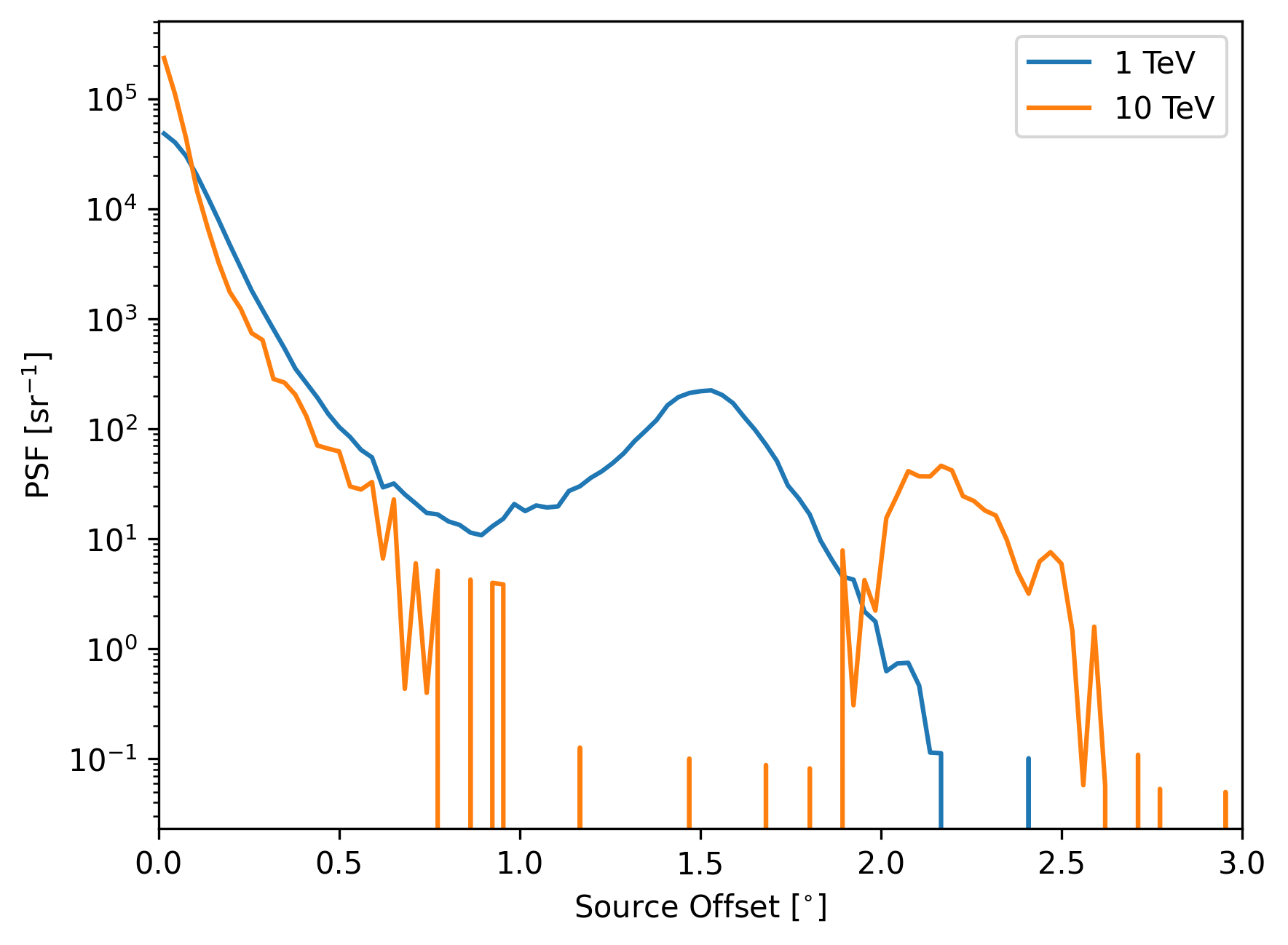
Point Spread Function

The point spread function describes how well the direction of the gamma rays is estimated.

from pyirf.irf import psf_table
from pyirf.utils import calculate_source_fov_offset


gammas['true_source_fov_offset'] = calculate_source_fov_offset(gammas)


source_offset_bins = np.linspace(0, 3, 100) * u.deg

# calculate this only for the events after the gamma/hadron separation
psf = psf_table(gammas[gammas['selected_gh']], true_energy_bins, source_offset_bins, fov_offset_bins)

psf.shape

(11, 1, 99)

Again, let’s use gammapy to plot:

from pyirf.gammapy import create_psf_3d

psf_gammapy = create_psf_3d(psf, true_energy_bins, source_offset_bins,  fov_offset_bins)

plt.figure()
psf_gammapy.plot_psf_vs_rad(offset=[wobble_offset], energy_true=[1., 10.]*u.TeV)
plt.legend(plt.gca().lines, ['1 TeV', '10 TeV'])

<matplotlib.legend.Legend at 0x7fde95d07040>

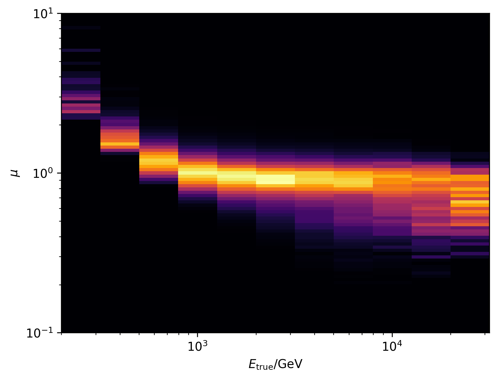
Energy Dispersion

Describes how well the energy is estimated

from pyirf.irf import energy_dispersion

# logarithmic space, is "symmetric" in terms of ratios 0.1 is a factor of 10 from 1 is a factor of 10 from 10
migration_bins = np.geomspace(0.1, 10, 100)

edisp = energy_dispersion(
    gammas[gammas['selected']],
    true_energy_bins=true_energy_bins,
    fov_offset_bins=fov_offset_bins,
    migration_bins=migration_bins,
)

Plot edisp

from gammapy.irf import EnergyDispersion2D

plt.figure()
plt.pcolormesh(
    true_energy_bins.to_value(u.GeV),
    migration_bins,
    edisp[:, :, 0].T,
    cmap='inferno'
)

plt.xlabel('$E_\mathrm{true} / \mathrm{GeV}$')
plt.ylabel('$\mu$')
plt.yscale('log')
plt.xscale('log')

Export to GADF FITS files

We use the classes and methods from astropy.io.fits and pyirf.io.gadf to write files following the GADF specification, which can be found here:

https://gamma-astro-data-formats.readthedocs.io/en/latest/

from pyirf.io.gadf import create_aeff2d_hdu, create_energy_dispersion_hdu, create_psf_table_hdu
from astropy.io import fits
from astropy.time import Time
from pyirf import __version__

# set some common meta data for all hdus
meta = dict(
    CREATOR='pyirf-v' + __version__,
    TELESCOP='FACT',
    INSTRUME='FACT',
    DATE=Time.now().iso,
)

hdus = []

# every fits file has to have an Image HDU as first HDU.
# GADF only uses Binary Table HDUs, so we need to add an empty HDU in front
hdus.append(fits.PrimaryHDU(header=fits.Header(meta)))

hdus.append(create_aeff2d_hdu(aeff_selected, true_energy_bins, fov_offset_bins, **meta))
hdus.append(create_energy_dispersion_hdu(edisp, true_energy_bins, migration_bins, fov_offset_bins, **meta))
hdus.append(create_psf_table_hdu(psf, true_energy_bins,    source_offset_bins, fov_offset_bins, **meta))

fits.HDUList(hdus).writeto('fact_irf.fits.gz', overwrite=True)